Machine Learning Algorithms

ML Algorithms with Python

    In this page I will discuss how and when to use certain machine learning algorithms when performing data analysis.

• Difference between Supervised & Unsupervised Learning?
• How to pick which algorithm to use?
• How to set up algorithm and scale data?
• What is a Training & Testing set?

This is my Github page where you can see implementation of most of these algorithms using Python.

Github

Algorithms in Machine Learning:

* I won't discuss all  of these Algorithms, only those that are commonly used.*

Supervised Learning

Supervised learning is a node of both machine learning and artificial intelligence methods. It is widely used to take datasets both simple & complex and train an algorithm to classify data (is the picture an apple or banana) or predict outcomes (stock prediction). 

Let's say we are given a data set with points of type x(1),..., x(n). Then we are also given a data set or single column of known outputs y(1) ,..., y(n). Our goal is to create a model that will learn how to predict the outcomes of x, which are y.

Linear Models:

We assume here that y|x; θ ∼ N (μ,σ2). By noting X the matrix design, the value of θ that minimizes the cost function is a closed-form solution such that:

Least Means Square:

By noting α the learning rate, the update rule of the Least Mean Squares (LMS) algorithm for a training set of m data points, which is also known as the Widrow-Hoff learning rule, is as follows:

Locally Weighted Regression:

This is a variant of linear regression that weights each training example in its cost function by w(i)(x), which is defined with parameter τ ∈ R as:

Logistic Regression:

We assume here that y|x;θ ∼ Bernoulli(φ). We have the following form:

Softmax Regression:

Also called a multiclass logistic regression, is used to generalize logistic regression when there are more than 2 outcome classes. By convention, we set θK = 0, which makes the Bernoulli parameter φi of each class i equal to:

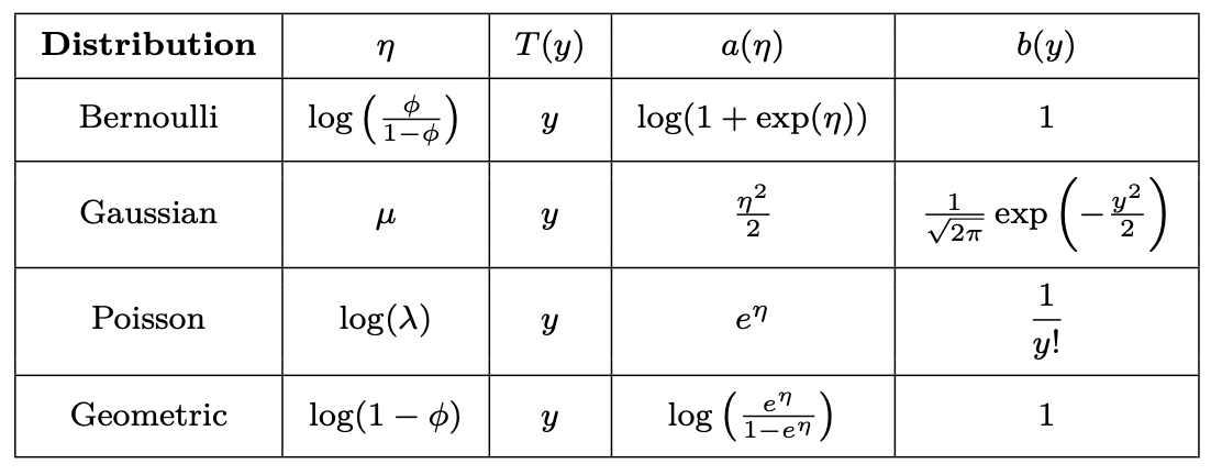
Exponential Models:

Most common exponential distributions summed up in the following table:

Support Vector Machines (SVM):

The main use of a SVM is to obtain a line that will maximize the minimum distance to a line of data.

The margin classifier (h) is given as:

This is only viable where (w, b) ∈ Rn × R is the solution of the following optimization problem. min 1/2||w||2 such that y(i)(wT x(i) − b) > 1.

Gaussian Discriminant Analysis:

The Gaussian Discriminant Analysis assumes that y and x|y = 0 and x|y = 1 are such that:

The following table sums up the estimates that we find when maximizing the likelihood:

Naive Bayes:

The Naive Bayes model supposes that the features of each data point are all independent:

Maximizing the log-likelihood gives the following solutions, with k ∈ {0,1}, l ∈ [1,L]. This method is usually for text classification and spam detection.

Random Forrest:

It is a tree-based technique that uses a high number of decision trees built out of randomly selected sets of features. Contrary to the simple decision tree, it is highly uninterpretable but its generally good performance makes it a popular algorithm.

K-nearest neighbors:

The k-nearest neighbors algorithm, commonly known as k-NN, is a non-parametric approach where the response of a data point is determined by the nature of its k neighbors from the training set. It can be used in both classification and regression settings.

Unsupervised Learning

Unsupervised learning is similar to the supervised method, but instead the data its being given is not labeled and the algorithms that are used are meant to discover hidden patterns or data groupings.

Clustering:

Latent variables are hidden/unobserved variables that make estimation problems difficult, and are often denoted z. Here are the most common settings where there are latent variables:

k-means clustering:

After randomly initializing the cluster centroids μ1,μ2,...,μk ∈ Rn, the k-means algorithm repeats the following step until convergence:

We note c(i) the cluster of data point i and μj the center of cluster j.

Hierarchical clustering:

It is a clustering algorithm with an agglomerative hierarchical approach that build nested clusters in a successive manner. There are different sorts of hierarchical clustering algorithms that aims at optimizing different objective functions, which is summed up in the table below:

Calinski-Harabaz Index:

By noting k the number of clusters, Bk and Wk the between and within-clustering dispersion matrices respectively defined as:

The Calinski-Harabaz index s(k) indicates how well a clustering model defines its clusters, such that the higher the score, the more dense and well separated the clusters are. It is defined as follows:

Principle Component Analysis:

Given a matrix A ∈ Rn×n, λ is said to be an eigenvalue of A if there exists a vector z ∈ Rn\{0}, called eigenvector, such that we have:

Let A ∈ Rn×n. If A is symmetric, then A is diagonalizable by a real orthogonal matrix U ∈ Rn×n. By noting Λ = diag(λ1,...,λn), we have:

Independent Component Analysis:

We assume that our data x has been generated by the n-dimensional source vector s = (s1,...,sn), where si are independent random variables, via a mixing and non-singular matrix A as follows:

The goal is to find the unmixing matrix W = A−1 by an update rule.

Probability / Likelihood / Stochastic Gradient

Important Statistics & Set-ups

Classification:

In a context of a binary classification, here are the main metrics that are important to track to assess the performance of the model The confusion matrix is used to have a more complete picture when assessing the performance of a model. It is defined as follows:

Regression:

Given a regression model f, the following metrics are commonly used to assess the performance of the model:

The coefficient of determination, often noted R2 or r2, provides a measure of how well the observed outcomes are replicated by the model and is defined as follows:

Model Selection:

When selecting a model, we distinguish 3 different parts of the data that we have as followed:

Once the model has been chosen, it is trained on the entire dataset and tested on the unseen test set. These are represented in the figure below:

Cross-validation, also noted CV, is a method that is used to select a model that does not rely too much on the initial training set. The most commonly used method is called k-fold cross-validation and splits the training data into k folds to validate the model on one fold while training the model on the k − 1 other folds, all of this k times. The error is then averaged over the k folds and is named cross-validation error.

Interpretation:

The bias of a model is the difference between the expected prediction and the correct model that we try to predict for given data points. The variance of a model is the variability of the model prediction for given data points. The simpler the model, the higher the bias, and the more complex the model, the higher the variance.

In all this page was an introduction/summary to most of the methods and algorithms in supervised and unsupervised machine learning. This was meant to explain the more hardcore mathematical approach on how these algorithms work, and how to alter them when conducting and creating your own machine learning algorithms and perhaps when to use one.

Please see my GitHub page on the implementation of machine learning algorithms using datasets found on the web.

Thank you,

Jose Hernandez